CMU 15-418 Parallel Computer Architecture and Programming

• Lecture 1. Why Parallelism
• Lecture 2. Instruction-Level Parallelism (ILP)
  • Pipelining
  • Out-of-Order (OoO) Execution
  • From ILP to Multicore
• Lecture 3. Modern Multi-Core Processor
  • Multi-Core
  • SIMD: Single Instruction Multiple Data
  • Hyperthreading (Simultaneous Multi-Threading, SMT)
  • Accessing Memory
  • Summary
• Lecture 4. Parallel Programming Abstractions and HW/SW Implementations
  • ISPC
  • Parallel Programming Models and Machine Architectures
• Lecture 5. Parallel Programming Basics
  • A Parallel Programming Example
• Lecture 6. Performance Optimization - Work Distribution and Scheduling
  • Work Assignment

Lecture 1. Why Parallelism

This is a class focusing on various of techniques of writing parallel programs. It consists of 4 labs that use different parallel strategies, including:

1. SIMD (Single Instruction Multiple Data) and multi-core parallelism;
2. CUDA (parallelism on GPU devices);
3. Parallelism via shared-address space model;
4. Parallelism via message-passing model.

The first lecture discusses the history of parallel programming and some performance advances in this field, such as:

1. Wider data paths/address bits: 4 bit -> … -> 32 bit -> 64 bit;
2. Efficient pipeline: lower Cycles per Instruction (CPI);
3. Instruction-level Parallelism (ILP) that detects independent instructions and execute them in parallel;
4. Faster clock rates: 10 MHz -> … -> 3GHz.

However, it’s more difficult to continue to advance ILP and clock rates due to the Power Density Wall.

On the hardware side, a transion has been happening from supercomputer to cloud computing, where the former focuses on lower latency and the latter more focuses on high throughput.

You can think latency means finishing a single task quickly whereas throughput means finishing more tasks in a period of time.

The formal definition of Parallel Computing: a collecitons of processing elements that cooperate to solve problems quickly. That means:

1. We need multiple processors to achieve parallelism;
2. These processors need to work in parallel to complete a task;
3. We care about performance/efficiency when using parallelism.

Parallelism v.s. concurrency: the two concepts are confusing. In my understanding, parallelism means, at a moment, multiple processors (e.g. cores) are working in parallel to complete a task(s). Concurrency only means there are multiple tasks/threads that are running. But they are not necessarily running in parallel but just interleaved. For example, OS may first start Task A and then put it in background and start Task B. After B is completed, OS continue to execute Task A.

This course uses speedup to measure parallelism when P processors are used, which is defined as the ratio of executing time by using 1 processor and the exectuing time by using P processors. Some potential issues when using parallelism and solutions inlcude:

1. Communication cost limits expected speedup (e.g., use P processors but only get P/2 speedup). Solution: minimize unnecessary communications.
2. Unbalanced work assignment limits expected speedup. Solution: balance workloads among processors to avoid any bottleneck.
3. Massive parallel execution that causes much higher communication cost compared to computation. (e.g., 100 cores to complete a simple task). Solution: partition the task to appropriate segmentations that are executable in parallel.

In summary, we need a parallel thinking that includes work decomposition, work assignment, and communication/syncronization management.

Lecture 2. Instruction-Level Parallelism (ILP)

Today’s topic is ILP, which is mainly used in CPUs and done in the hardware level. But first, let’s discuss the different parallelism strategies between two popular chips, CPU and GPU: in CPU, parallelism is incorporated into hardware-level, which dynamically schedules instructions, so it’s not (relatively) difficult to write parallel program on CPUs; however, parallelism on GPUs is done in software level, meaning programmers have to explicitly write code to handle/specify how to parallel the computation.

This also leads to different hardware design: CPU usually has only few powerful cores (tens) and most of the chip area is used for scheduling/communication (finding parallelism); in GPU, there is many simple cores (thousands). And softwares/programs are responsible for scheudling parallel execution (e.g., CUDA).

Let’s back to ILP and see some ideas that CPUs use to speed up sequential code, including:

1. Pipelining & Superscalar: work on multiple instructions at once;
2. Out-of-Order (OoO) execution: dynamically schedule instructions (via dataflow graph);
3. Speculation: predict the next instruction to discover more independent work and roll back on incorrect predictions.

All these techniques are implemented within the hardware, which is invisible to software. And in the software level, all instructions are still executed in-order, one-at-a-time.

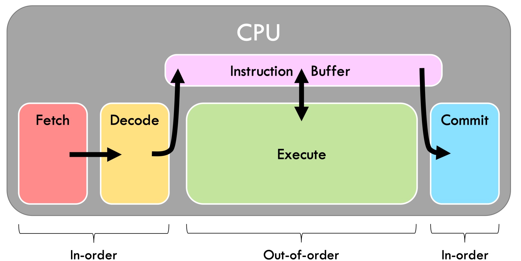
First we define a simple CPU model which executes instruction in sequential, and assume an instruction execution is divided in to four stages:

1. Fetch: read the next instruction from memory;
2. Decode: figure out what to do and read inputs;
3. Execute: perform operations on ALU;
4. Commit: write results back to registers/memory.

Suppose each stage costs 1ns, such a model has a latency of 4ns/instruction and a throughput of 0.25instruction/ns.

Latency: time spent to complete a job (request, instruction, etc). Throughput: number of jobs completed per time unit (1ns, 1day, etc).

Pipelining

Pipelining executes multiple instructions that are in different stages in parallel. But it is still in-order execution and just keep fetching new instructions whenever possible.

It enables ILP by starting the next instruction immediately when the corresponding stage processor is available. Also since it’s ILP, the latency of each instruction keeps unchanged (4ns/instruction). However, the throughput is improved 4 times, to 1instructions/ns(ideally). Because we have 4 stages, we can parallel 4 instructions at maximum.

One limitation of pipelining is that it requires independent work, meaning no read-after-write conflict. This introduces data hazard because mostly instructions are interrelated, especially those next to each other.

Solutions:

1. Stalling pipeline: when there is a read-after-write conflict, stall the pipeline to avoid to read the wrong value;
2. Forwarding data: after the write operation is done, it forwards the new value direclty to the next read instruction so that the read instruction doesn’t need to wait until write is committed.

Forward data is expensive, especially in deep & complex pipelines.

Another limitation of pipelining is control hazard: we pipeline instructions sequentially, but branches (goto, while, for) redirect execution to new location, making us fetch the wrong instructions.

Solutions:

1. Flushing pipeline: execute instructions sequentially. When there is an error, flush the wrong instructions and jump to the correct place;
2. Speculation: predict where to go next and execute instructions in the predicted place (can use ML to predict branches).

Flush is also expensive in deep pipelines. For example, in nested loops, instruction errors happen more frequently.

Out-of-Order (OoO) Execution

Think of OoO execution as a topological sort on a dataflow graph.

Different from pipelining where we ensure instructions are executed in-order, OoO execution only ensures correct dataflow/true data dependency and thus avoid unnecessary data dependency (write-after-read, read-after-read).

Dataflow increases parallelism by eliminating unnecessary dependences.

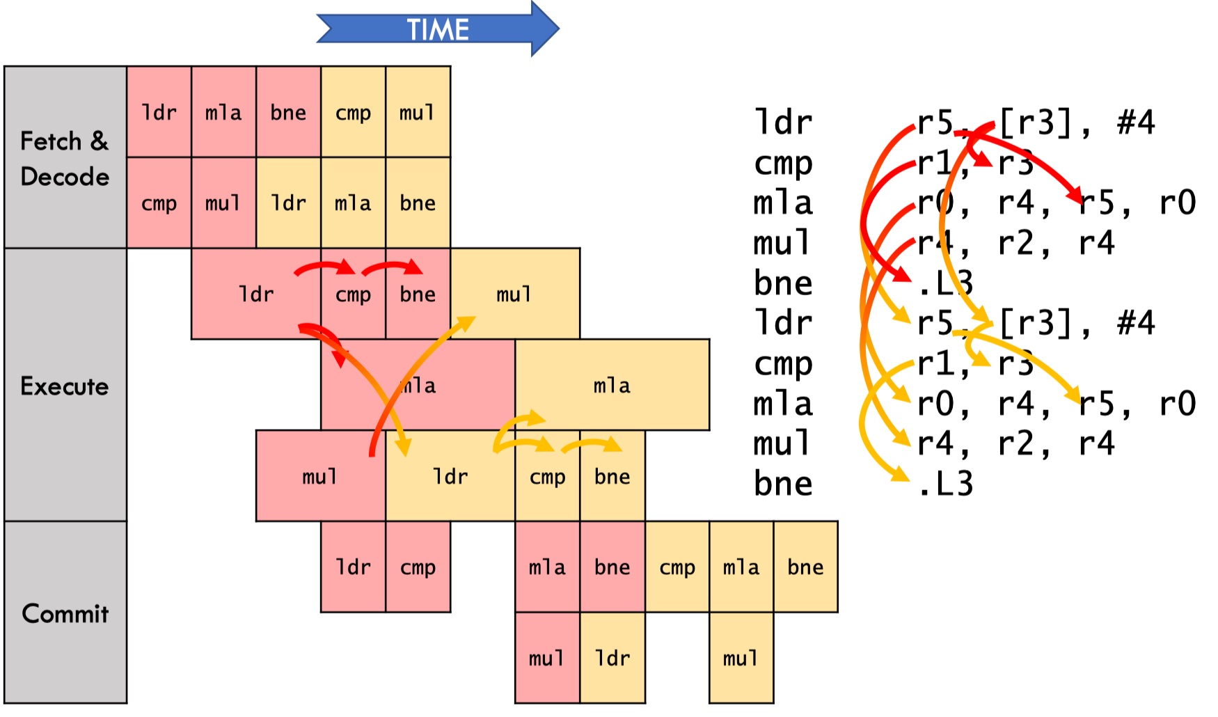
The first performance bottleneck in OoO is Latency-bound, in which lantency is bounded by a specific operation/instruction, making it unable to further improve latency. We can find the latency bound of a computation by its cretical path, which is the longest path across iterations in a dataflow graph.

With the above chip, a program is now throughput-bounded. That is because we can only execute 1 instruction at a time with a single execute unit (fetch and commit usually don’t limit performance).

Superscalar OoO is the solution to unleash throughput-bound. It increase pipeline width by using multiple execution units, such that execution no longer limits performace (only dataflow does).

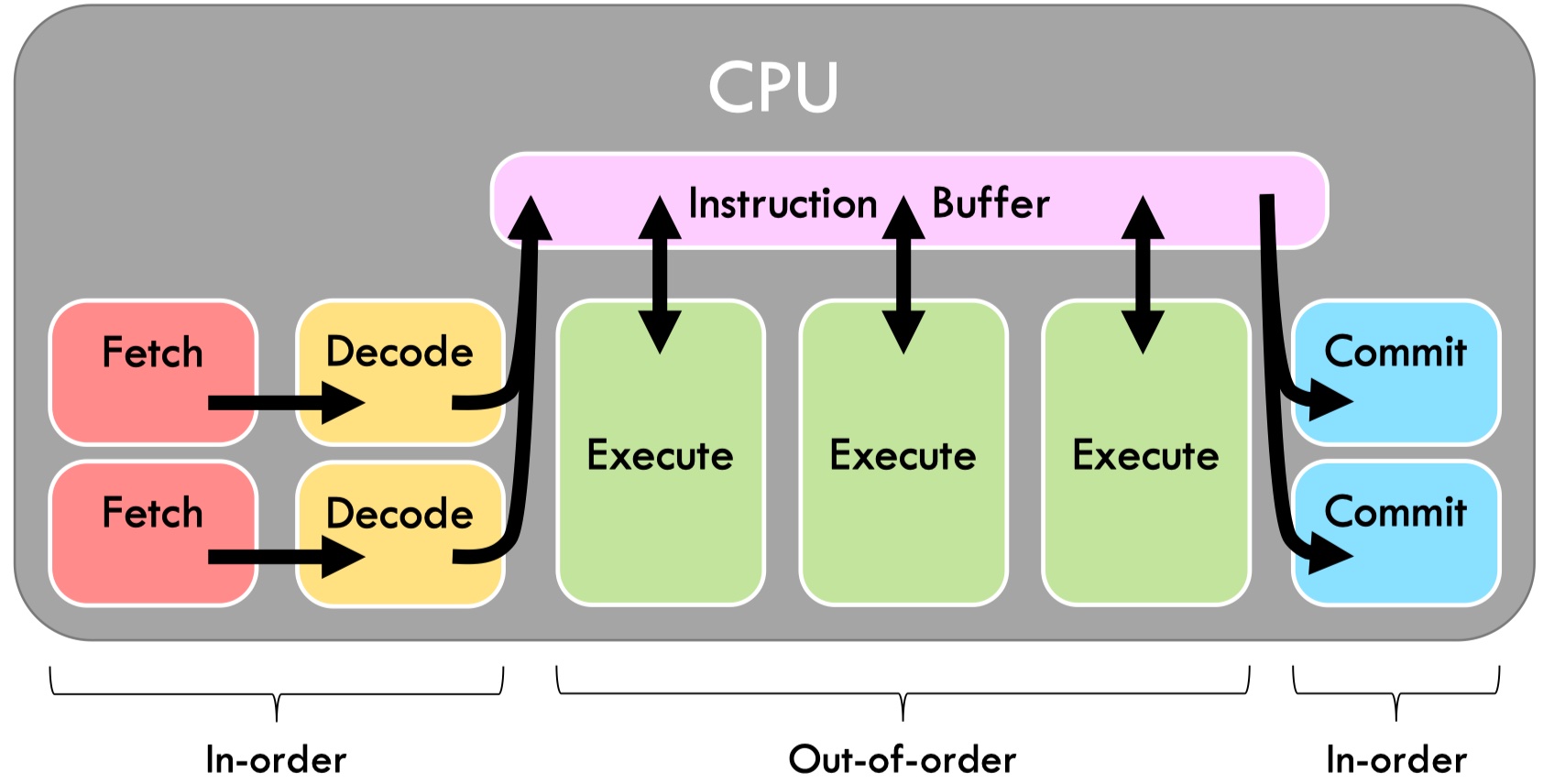
Another throughput limitation is structural hazards, which means data is ready but instructions cannot be executed because no hardward is available. A chip only contains limited numbers of different types of execution units such as floating-point units, interger units, etc.

Register renaming: OoO processors eliminate false dependences (write-after-read, write-after-write) by transparently renaming registers.

From ILP to Multicore

ILP hasn’t gotten large boosts recently. One reason is that superscalar scheduling is complex. For example, to decide if it should issue two instructions, the CPU needs to compare all pairs of input/output registers to check if there is a read-after-write conflict.

Nowadays multicore is a more preferred choice where each core might become simpler. However, writing parallel software is still hard.

Lecture 3. Modern Multi-Core Processor

Today’s lecture discusses some thread-level parallelism that usually involves multiple instruction streams, including multi-core, SIMD, super-threading.

Different from ILP in which most of the work is done by hardwards, multi-threading parallelism requires writing multi-thread softwares.

This lecture uses a code example to demonstrate how it can be parallelized by these techniques.

// Calculate sin(x) for N numbers starting at `x`, using Tayler expansion.
void sinx(int N, int terms, float *x, float *result) {
  for (int i = 0; i < N; i++) {           // outer-loop, independent between different i
    float value = x[i];
    float numer = x[i] * x[i] * x[i];
    int denom = 6;  // 3!
    int sign = -1;

    for (int j = 1; j <= terms; j++) {    // inner-loop
      value += sign * numer / demon;
      numer *= x[i] * x[i];
      denom *= (2 * j + 2) * (2 * j + 3);
      sign *= -1;
    }

    result[i] = value;
  }
}

With ILP, the only possible parallelism is that a processor can execute multiple instructions by using pipelining (in-order) or superscalar (OoO).

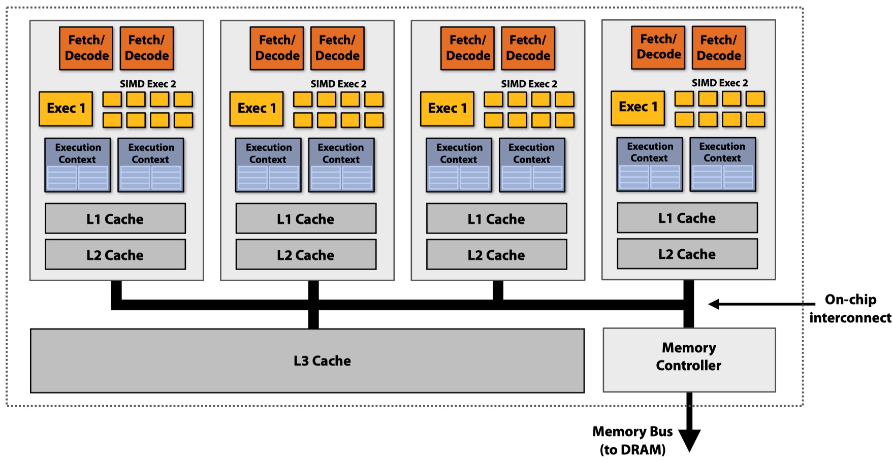
Multi-Core

Use increasing transistor count to add more cores to the processor.

The transition from a single powerful core to multiple simple cores also leads to different hardware design strategies. In single-core processor, more transistors are used to speed up a single instruction stream (e.g. larger cache, smart OoO logic and branch predictor). Now more transistors are used to add more cores or other parallelism units (e.g., SIMD ALU).

The challenge is how we can write parallel programs that can fully utilize these multi cores. One solution is using multi-threads in which we explicitly creates multiple threads (e.g. pthreads) can assign the work evenly to these threads. The disadvantage is that we need to hardcode the number of threads created, which is usually dependent on hardwares.

typedef struct { int N; int terms; float* x; float* result; } my_args;

void parallel_sinx(int N, int terms, float* x, float* result) {
  pthread_t thread_id; 
  my_args args;
  args.N = N/2;
  args.terms = terms; 
  args.x = x; 
  args.result = result;

  pthread_create(&thread_id, NULL, my_thread_start, &args); // launch thread 
  sinx(N - args.N, terms, x + args.N, result + args.N); // do work 
  pthread_join(thread_id, NULL);
}

void my_thread_start(void* thread_arg) {
  my_args* thread_args = (my_args*)thread_arg;
  sinx(args->N, args->terms, args->x, args->result); // do work 
}

We can also use data-parallel expression where we just anotate the code blocks that are data-parallel (e.g., independent loops) using language-specific notations and let the compiler generate parallel threaded code. The benefit is that the compiler can decide how many threads created based on the hardware that runs the program.

void sinx(int N, int terms, float *x, float *result) {
  forall (int i from 0 to N-1) {           // data-parallel expression
    float value = x[i];
    float numer = x[i] * x[i] * x[i];
    int denom = 6;  // 3!
    int sign = -1;

    for (int j = 1; j <= terms; j++) {    // inner-loop
      value += sign * numer / demon;
      numer *= x[i] * x[i];
      denom *= (2 * j + 2) * (2 * j + 3);
      sign *= -1;
    }

    result[i] = value;
  }
}

One common thing is that after the work is divided and assigned to different threads, we can execute these threads in parallel on different cores.

SIMD: Single Instruction Multiple Data

Add more ALUs within a core to amortize cost/complexity of managing an instruction stream across many ALUs.

SIMD is a technique that execute the same instruction stream in parallel on all ALUs using multiple data. The idea is that in some situations such as vector calculation or for-loop, we do the same operations (instructions) on multiple data sources. So we can just use multiple ALUs within a core (one ALU per data source) and execute this instruction stream on all data source in parallel.

Similar to data-parallel expression, SIMD also uses language-specific anotations to generate parallelism code. Some examples includes AVX and CUDA.

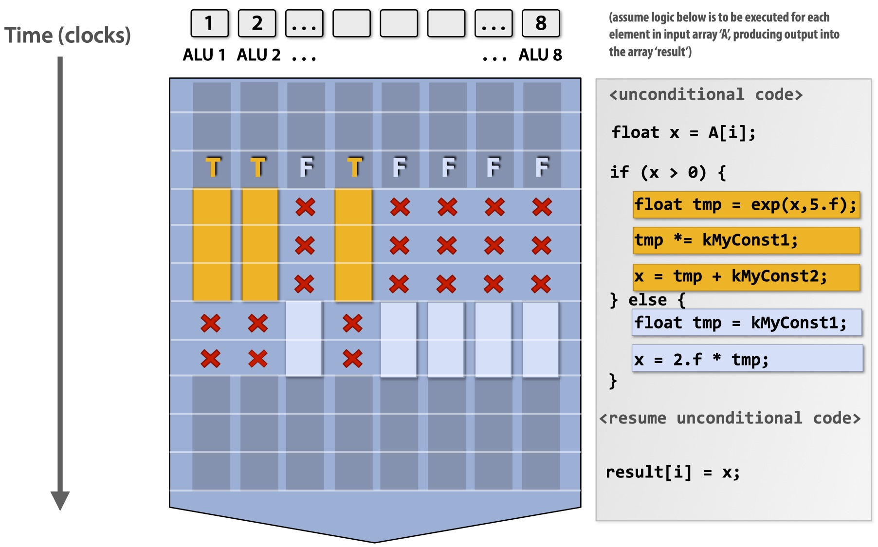
One issue of SIMD is conditional execution where the code is the same but execution not depending on the condition values (e.g., if-else statement). SIMD resolves the issue by using mask. It first calculates a mask for each data source based on the condition expression. Then it executes both if and else but disables the effect of one of them, depending on the mask value.

Mask hurts parallelism performance since it wastes computations.

Coherent execution (instruction stream coherence): same instruction sequence applies to all elements operated upon simultaneously.

Coherent execution is required for efficient SIMD implementation, not required for multi-core parallelization. It makes sense because each core has its own fetch/decode units while SIMD only requires multiple ALUs within a core.

SIMD on Modern Hardwares

CPUs mainly use explicit SIMD where SIMD parallelization is performed at compile time and instructions are generated by compiler. That means you can check the progrm to see which SIMD instruction are used. Some CPU SIMDs includes:

• SSE instructions: 128-bit operations: 4x32 bits or 2x64 bits (4-wide float vectors),
• AVX instructions: 256-bit operations: 8x32 bits or 4x64 bits (8-wide float vectors),
• AVX512 instructions: 512-bit operations: 16x32 bits or 8x64 bits (16-wide float vectors).

As a comparision, GPUs use implicit SIMD where the compiler only generates a scalar binary (scalar instructions, no SIMD yet). Then the hardware executes the same scalar instructions simultaneously from multiple data source on SIMD ALUs. The programmer only needs to define SIMD by using a data-parallel interface (e.g., execute(my_func, N);).

Hyperthreading (Simultaneous Multi-Threading, SMT)

Perform multi-threading using superscalar hardware within a core: fetch/decode instructions from different threads and execute them OoO within a core.

Accessing Memory

Memory latency: amount of time for a memory request (e.g., 100 cycles); memory bandwidth: rate at which the memory can provide data to a processor (e.g., 20 GB/s).

Caches can reduce latency by reducing stall lengths (faster access). Prefetching (discussed in lecture 2 - pipelining) can hide latency by utilizing some stalls to prefetch instructions. Multi-threading also hides lantency by interleave processing multiple threads.

With thread-level parallelism, we are moving to a throughput-oriented system: the goal is to increase overall system throughput when running multiple threads, althought individual work might need more time to complete.

Bandwidth-limited: in throughput-optimized systems, if processors request data at a too high rate (GPU), the memory system cannot keep up. Some mitigations include:

1. Reuse data previously loaded by the same thread.
2. Share data across threads.
3. Request data less often (instead, do more arithmetic).

Arithmetic intensity: ratio of math operations to data access operations in an instruction stream.

Summary

This lecture introduces three parallelism techniques:

• Multi-core: thread-level parallelism, run one thread per core in parallel.
  • Require multi-core processor.
• SIMD: execute the same instruction stream on multiple data sources in parallel within a core.
  • Require multiple ALUs within a core.
• Hyperthreading: run multiple threads using superscalar harware within a core.
  • Require OoO superscalar hardware.

Lecture 4. Parallel Programming Abstractions and HW/SW Implementations

This lecture first compares abstractions and implementations, with ISPC as an example. Then three parallel programming models are discussed, including:

1. Shared-memory model;
2. Message-passing model;
3. Data-parallel model.

ISPC

ISPC is a SPMD (Single Program Multiple Data) programming abstraction based on SIMD. Programers write code in SPMD and the ISPC compiler generates SIMD implementations. With ISPC/SPMD, programmers don’t need to write complicated code with SIMD vector ops.

When using ISPC, the programmer need to write C-like functions in .ispc files. Then calling to ISPC functions will spawns “gang” of ISPC programming instances to run ISPC code concurrently, and return when all instances complete. Below is the same sin(x) example but implemented in ISPC. Compare this code with the AVX vector implementation and see how SPMD helps reduce the complexity of SIMD.

// ----- main.cpp
#include "sinx_ispc.h"

int N = 1024;
int terms = 5;
float *x = new float[N];
float *res = new float[N];

// init x here

// exec ISPC code
sinx(N, terms, x, res);

// ----- sinx.ispc
export void sinx(
  uniform int N,
  uniform int terms,
  uniform float *x,
  uniform float *result
) {
  // assume N % programCount == 0
  for (uniform int i = 0; i < N; i += programCount) {
    int idx = i + programIndex;
    float value = x[idx];
    float numer = x[idx] * x[idx] * x[idx];
    uniform int denom = 6 // 3!
    uniform int sign = -1;

    for (uniform int j = 1; j <= terms; j++) {
      value += sign * numer / denom;
      numer *= x[idx] * x[idx];
      denom *= (2*j+2) * (2*j+3);
      sign *= -1;
    }

    result[idx] = value;
  }
}

When this code is executed, only the ISPC function is executed concurrently and all other C codes are sequential execution. Notice the ISPC keywords such as programCount and programIndex in ISPC functions:

1. programCount: number of simultaneously executing instances in a gang (uniform value);
2. programIndex: id of the current instance within the gang (non-uniform value, [0, programCount));
3. uniform: type modifier indicating that, within loop, all instances will have the same value for this variable. Its use is purely for optimization (e.g. all gangs can share the same one instead of creating programCount variables).

ISPC Instance Assignment

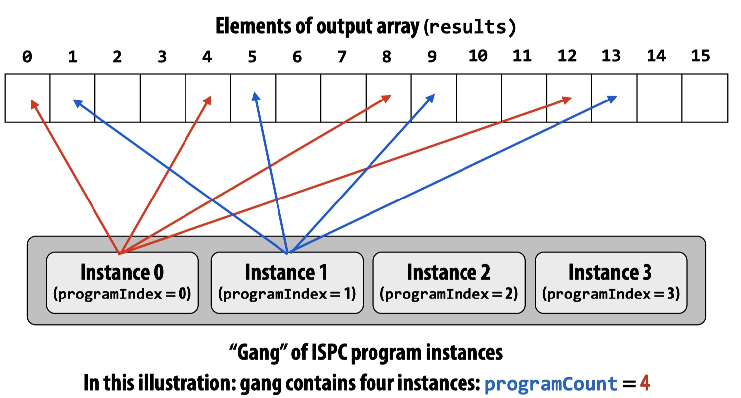
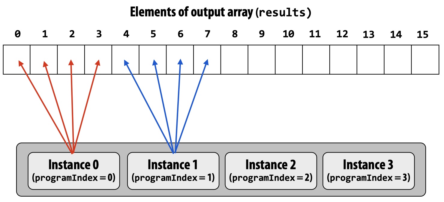
We can write ISPC code to control the assignment ISPC instances in a gang. The above example generate interleaved assignment of ISPC instances. We can also write similar code that has blocked assignment:

// main.cpp is the same

// sinx.ispc
export void sinx(
  uniform int N,
  uniform int terms,
  uniform float *x,
  uniform float *result
) {
  // assume N % programCount == 0
  uniform int count = N / programCount;   // each instance does `count` loops
  int start = programIndex * count;       // each instance starts at `start`
  for (uniform int i = 0; i < count; i++) {
    int idx = start + i;
    float value = x[idx];
    float numer = x[idx] * x[idx] * x[idx];
    uniform int denom = 6;
    uniform int sign = -1;

    for (uniform int j = 1; i <= terms; j++) {  // same inner-loop
      value += sign * numer / denom;
      numer *= x[idx] * x[idx];
      denom *= (2*j+2) * (2*j+3);
      sign *= -1;
    }

    result[idx] = value;
  }
}

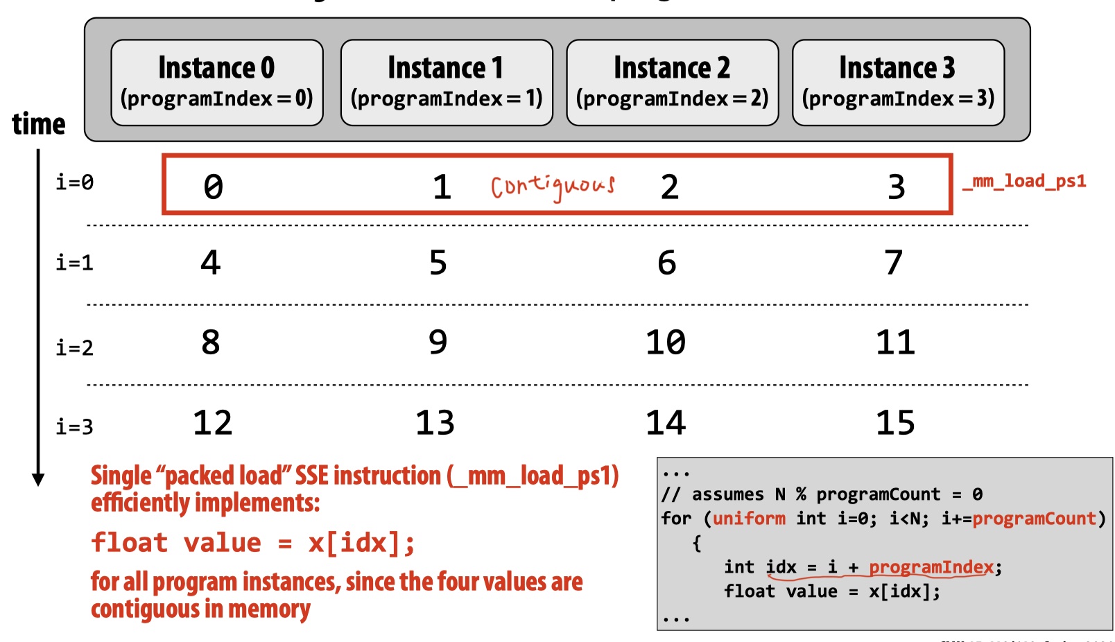
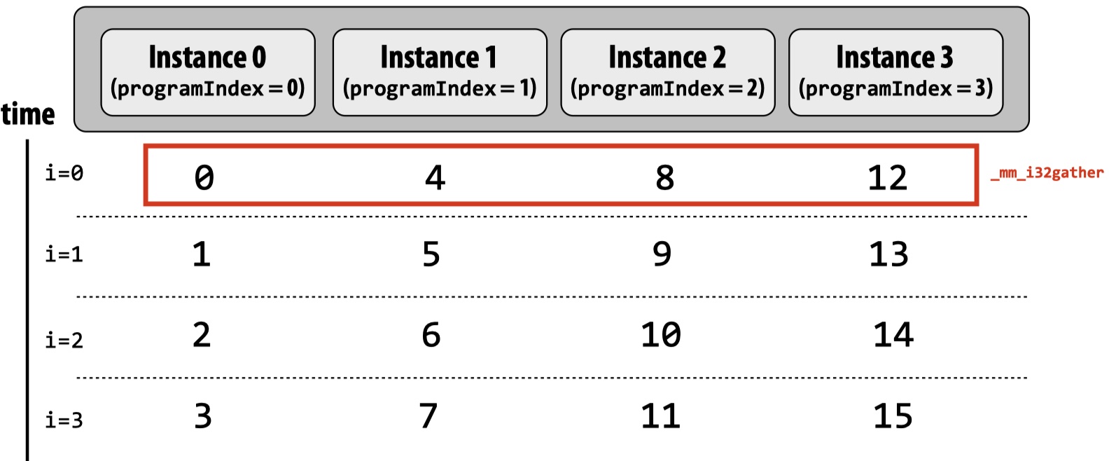
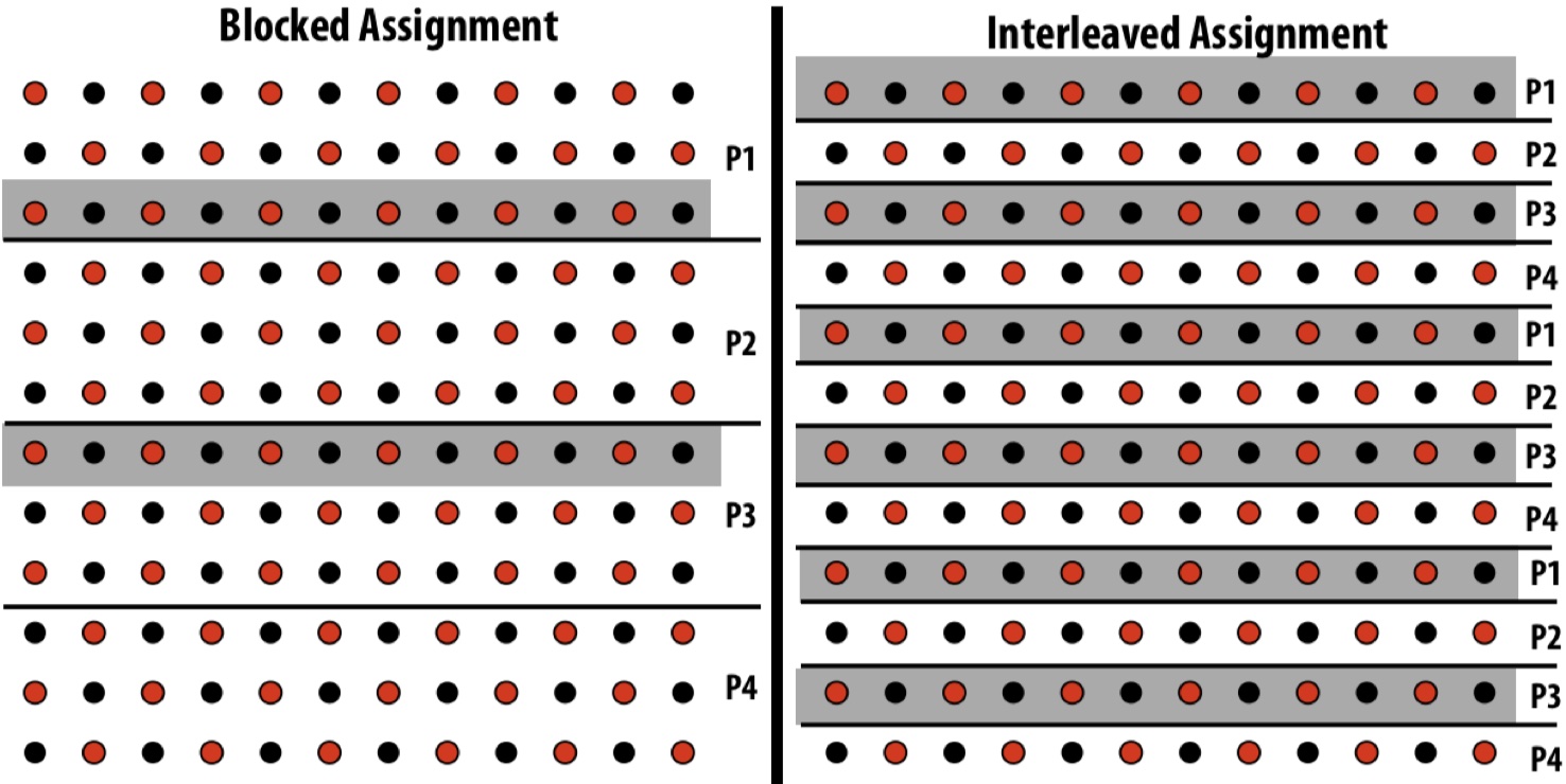
Below is a visualization of the two different instance assignments. To compare which one is better, we also need to dive into how each loop is scheduled among each instance across time. From figure we can see that, in each batch, the interleaved assignment reads/writes contiguous values (0, 1, 2, 3) but the blocked assignment doesn’t (0, 4, 8, 12). Remember ISPC/SPMD is still based on SIMD. SIMD has efficient operation implementations for contiguous values (e.g., packed load _mm_load_ps1). With blcoked assignment, SIMD now touch programCount non-contiguous values in memory, which is usually done by more costly operations such as gather.

Raising Abstraction Level with foreach

In previous examples, we still need to use ISPC keywords to decide the number of parallel-exection instances (programCount) and index individual instances (programIndex). foreach is a key ISPC language construct which declares parallel loop iterations. Then ISPC assigns iterations to program instances in gang and performs a static interleaved assignment by default.

// sinx.ispc
export void sinx(
  uniform int N,
  uniform int terms,
  uniform float *x,
  uniform float *result
) {
  foreach (i = 0 ... N) {
    float value = x[i];
    float numer = x[i] * x[i] * x[i];
    uniform int denom = 6;
    uniform int sign = -1;

    for (uniform j = 1; j <= terms; j++) {
      value += sign * numer * denom;
      numer *= x[i] * x[i];
      denom *= (2*j+2) * (2*j+3);
      sign *= -1;
    }

    result[i] = value;
  }
}

ISPC gang abstraction is implemented by SIMD instructions on one core, thus no multi-core parallelism. ISPC also provides a Task abstraction (similar to thread but more light weight) that achieves multi-core parallelism.

Parallel Programming Models and Machine Architectures

The programming models differ in communication and cooperation abstractions to programmers, which leads to different machine architectures.

Shared Address Space

Threads communicate by reading/writing to shared variables (visible to any thread) and manipulating synchronization primitives (e.g. lock, to ensure mutual exclusion).

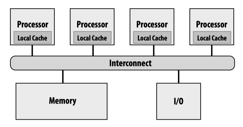
HW implementation support: any processor can directly reference any memory location. Two HWs that satisfy this requirement are Symmetric (shared-memory) multi-processor (SMP) and Non-uniform memory access (NUMA).

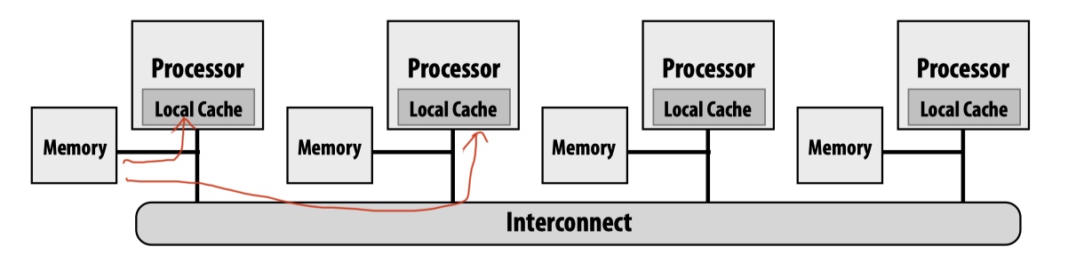
By exploiting memory locality, NUMA is usually more scalable than SMP. Even with NUMA, however, shared address space model still suffers from scalability. Cache coherence is a big issue.

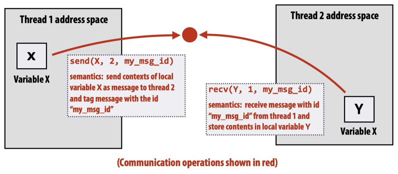
Message Passing

Different from shared address space model, in message passing model each threads operate within their private address spaces and only communicate by sending/receiving messages.

The benefit of message passing is that it doesn’t require HW implementations of system-wide loads/stores. It can also be used for clusters.

Data Parallel

Data parallel usually means applying the same operations on each elememnt of an array (often through SPMD).

map(function, collection) foreach in ISPC is an example of data parallel.

Stream programming model is a form of data parallel in which kernels are applied to each element in a stream.

• Stream: collections of elements, each of which can be processed independently;
• Kernel: pure-function that is applied to each element of a stream.

Lecture 5. Parallel Programming Basics

This lecture is mainly to go through the three parallel programming models discussed in the last lecture based on an example, grid solver.

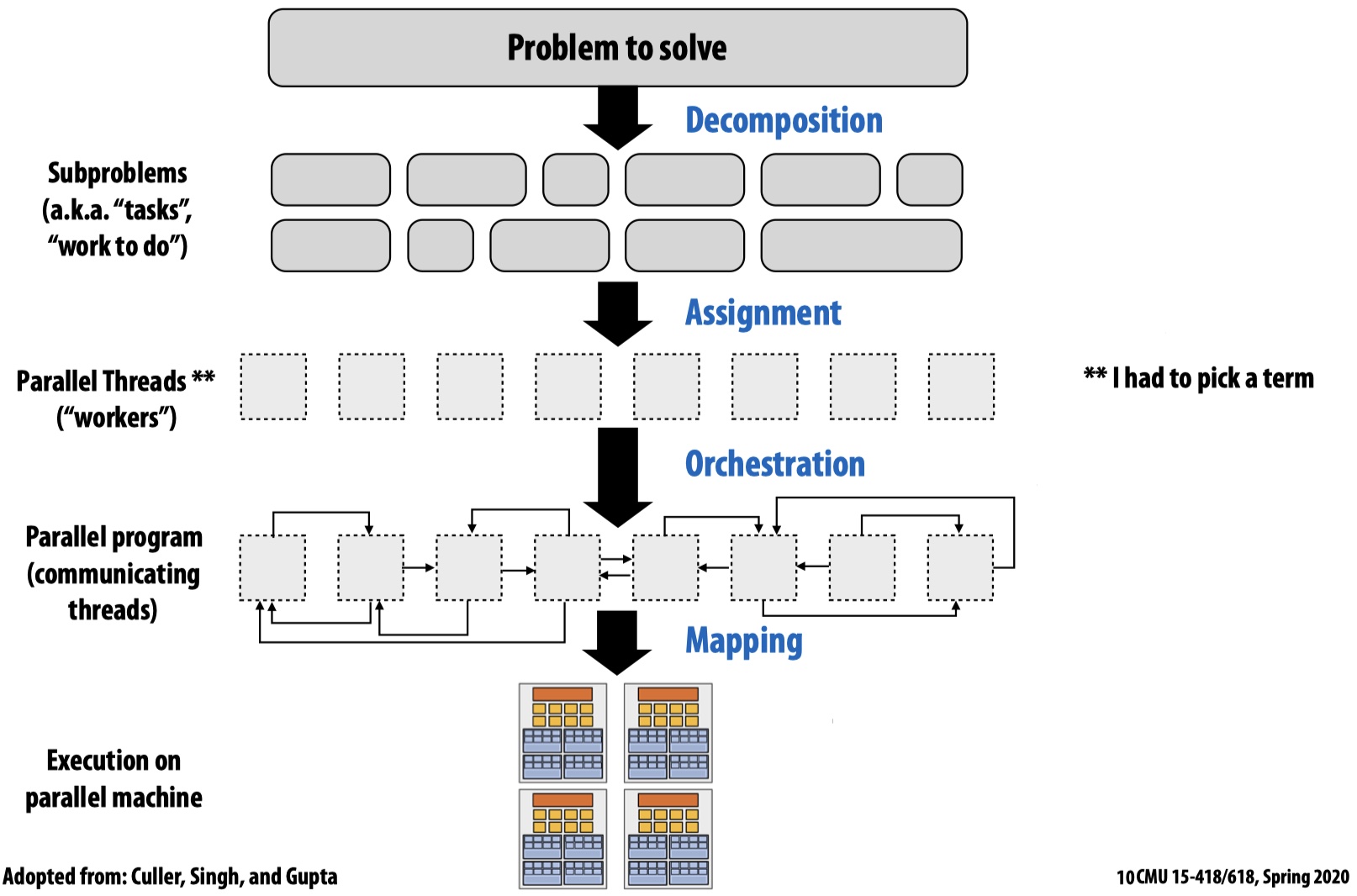
In practice, creating a parallel program involves 4 steps: decomposition (to create independent tasks), assignment (assign tasks to workers), orchestration (to coordinate processing of tasks by workers), mapping (tasks to hardware), each of which may be done by programmers or by system (compiler, runtime, hardware), depending on the specific parallelism mechanism used.

Decomposition is to break up a problem into tasks that can be carried out in parallel. The main idea is to create at least enough tasks to keep all execution units busy. The key is to indentify dependencies such that the decomposition will not affect the correctness of the original program.

Assignment is to assign tasks to threads/workers. The goal is to balance the workload and reduce communication costs.

Assignment can be done statically (e.g. via hardcode programCount or via pthread syscall) or dynamically during execution (e.g. foreach statement in ISPC).

Dynamic assignment is usually done by runtime (e.g. compiler) not programmer, which leads to simple and clean code. Also the runtime can generate different assignments based on given hardwards. However, it also requires extra space (e.g. extra data structures) and runtime (extra computations) costs.

As an example, ISPC tasks runtime stores all tasks in a list and whenever a worker completes a task, it inspects the list and assigns itself a new task from the list.

Orchestration is mainly to chain parallel executions, consisting of structring communication, adding synchronization (to preserve dependencies), organizing data structures, scheduling tasks, etc. The goal is to reduce communication/synchronization costs, preserve data locality, reduce overlead, etc.

Mapping means mapping threads/workers to hardware execution units, which can be done by OS (pthread -> CPU), by compiler (ISPC instances -> SIMD ALU), by hardware (CUDA -> GPU).

A Parallel Programming Example

Solve partial differential equation (PDE) on a (N+2)*(N+2) grid, using the iterative Gauss-Seidel solution until convergence. The sequential implementation is given:

const int n;
float *A;         // Store the `(N+2)*(N+2)` grid

void solve(float *A) {
  float diff, prev;
  bool done = false;

  while (!done) {
    diff = 0.0;
    for (int i = 1; i <= n; i++) {
      for (int j = 1; j <= n; j++) {
        prev = A[i,j];
        A[i,j] = 0.2 * (A[i,j] + A[i,j-1] + A[i-1,j] + \
                        A[i,j+1] + A[i+1,j]);      // Gauss-Seidel
        diff += abs(A[i,j] - prev);
      }
    }

    if (diff / (n * n)) < TOLERANCE)
      done = true;
  }
}

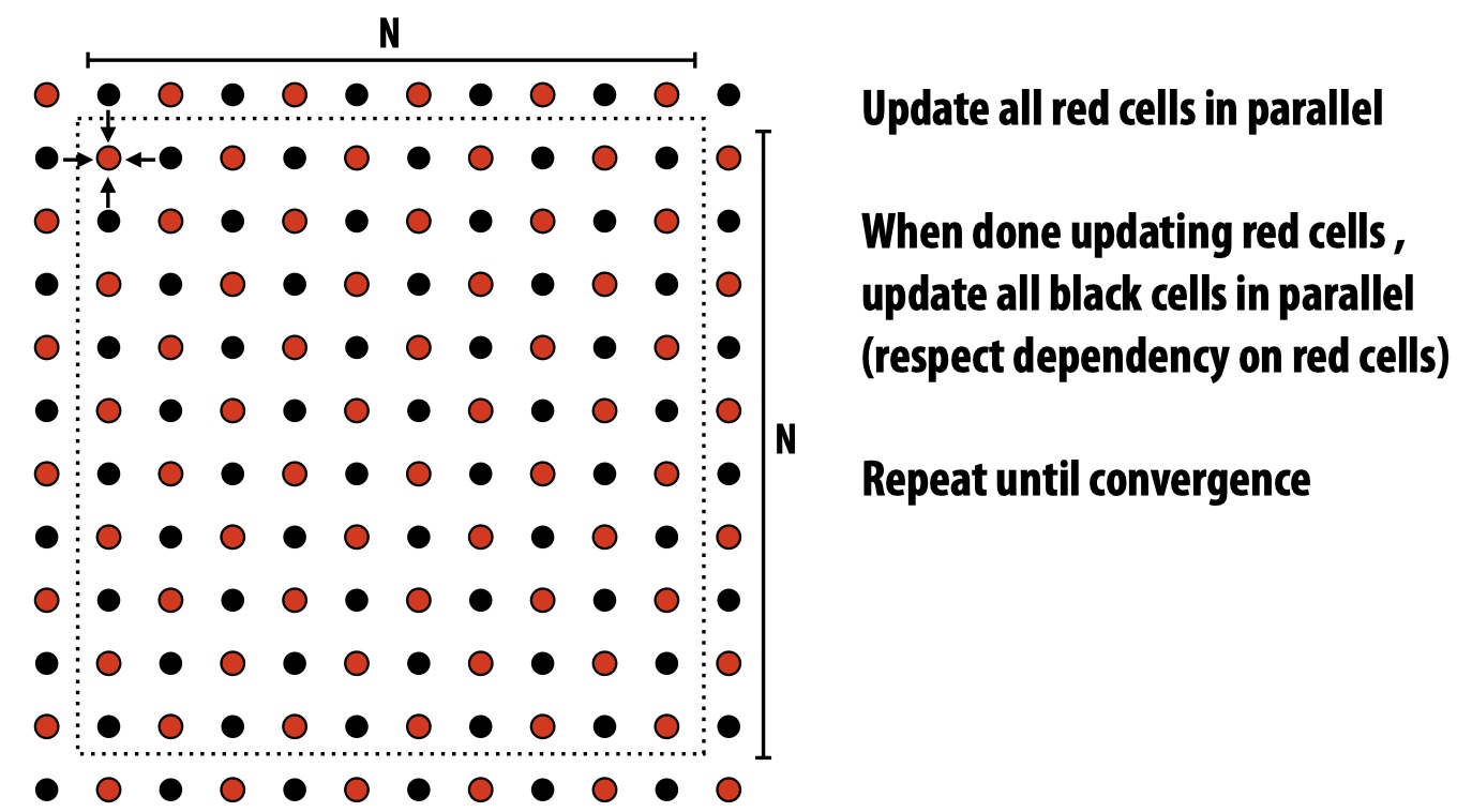
To improve the parallelism by reducing data dependencies. We instead use an approximation method (red-black coloring) that interleaves grid cell updates to two batches (red, black), in a way such that cells with the same color don’t have dependencies and thus can be updated in parallel.

Next is the assignment step. The below figure shows that, given this example, block assignment requires less data communication between processors compared to interleaved assignment.

After the assignment, we can implement the parallel grid solver using the three parallel programming models.

Here we only show red-cell update. Black-cell is similar.

Data-Parallel

In most cases, data-parallel model leads to simple and clean code since the programmer can write code similar to single-worker code. The library runtime (or hardware) will be responsible for parallel steps such as assigning tasks to individual workers, etc. For example, in the given implementation below,

const int n;
float *A = allocate((n + 2) * (n + 2));

void solve(float *A) {
  bool done = false;
  float diff = 0.0;

  while (!done) {
    foreach(j if red_cell(i, j)) {          // a. Decomposition
      float prev = A[i,j];
      A[i,j] = 0.2 * (A[i-1,j] + A[i,j-1] + A[i,j] + \
                      A[i+1,j] + A[i,j+1]);
      reduceAdd(diff, abs(A[i,j] - prev));  // b. Orchestration
    }                                       // c. Orchestration

    if (diff / (n * n) < TOLERANCE)
      done = true;
  }
}

all red cells (i, j) are independent tasks that can be parallelized (step a). Both b and c are orchestration steps handled by the system (e.g. ISPC). b involves built-in communication primitives whereas c is the end of foreach block which will implicitly wait for all workers before returning to sequential control.

Shared Address Space (via SPMD Threads)

Shared address space model requires programmers to handle synchronization by using primitives such as Lock (to provide mutual exclusion) and Barrier (to wait for threads before proceeding, similar to waitAll in some languages).

Barrier is used to ensure that dependencies are not violated due to parallelism and data sharing.

Three things to notice in the below implementation:

1. In shared memory address space model, the programmer is responsible to assign tasks to workers.
2. To reduce lock usage, we use partial sum in each thread and combine them at the end.
3. Three Barrier are used for different purpose:
   • b1: ensure diff clear is completed.
   • b2: ensure local diff computation (in current iteration) is completed.
   • b3: ensure global diff comparision is done before clearing them.

Using another trick can reduce Barrier from 3 to 1. The idea is using 3 different copies of global diff such that there is no dependencies between successive loop iterations.

// Assume these are global variables
// visible to all threads.
int n;
float *A = allocate((n + 2) * (n + 2));
bool done = false;
float diff = 0.0;
Lock myLock;
Barrier myBarrier;

void solve(float *A) {
  int tid = getThreadId();
  float myMin = (1 + tid * n / NUM_PROCESSORS); // Block assignment.
  float myMax = myMin + n / NUM_PROCESSORS;

  while (!done) {
    float diff_i = 0.0;   // Local diff to reduce lock usage.
    diff = 0.0;
    barrier(myBarrier, NUM_PROCESSORS);         // b1.
    for (int i = myMin; i < myMax; i++) {
      for (int j: red_cell(i, j)) {
        float prev = A[i,j];
          A[i,j] = 0.2 * (A[i-1,j] + A[i,j-1] + A[i,j] + \
                          A[i+1,j] + A[i,j+1]);
          diff_i += abs(A[i,j] - prev);
      }
    }

    lock(myLock);   // Combine local sums.                         
    diff += diff_i;
    unlock(myLock);

    barrier(myBarrier, NUM_PROCESSORS);       // b2.
    if (diff / (n * n) < TOLERANCE)
      done = true;
    barrier(myBarrier, NUM_PROCESSORS);       // b3.
  }
}

Message-Passing

In message-passing model, after the blocked assignment, each worker owns the assigned block as its private address space. All the memory sharing (e.g. rows in the block boundaries) need to be done as sending/receiving messages.

For simplicity, we give each block two rows of “ghost cells” that receive and store the boundary cell data from neighboring workers. And in each iteration, the two neighboring blcoks will send the required row to this block.

// Assume all initializations are done here.
int n;
int tid = getThreadId();
int rowPerThread = n / getNumThreads();
float *localA = allocate((rowPerThread + 2) * (N + 2));

void solve() {
  bool done = false;
  while (!done) {
    float myDiff = 0.0;

    // 1. Communication (send/recv ghost rows).
    if (tid % 2) {
      sendDown(); recvDown();
      sendUp();   recvUp();
    } else {
      sendUp();   recvUp();
      sendDown(); recvDown();
    }

    // 2. Main computation.
    for (int i = 0; i < rowsPerThread + 1; i++) {
      for_all(red_cell(i,j)) {
        float prev = A[i,j];
          A[i,j] = 0.2 * (A[i-1,j] + A[i,j-1] + A[i,j] + \
                          A[i+1,j] + A[i,j+1]);
          diff_i += abs(A[i,j] - prev);
      }
    }

    // 3. Communication/Synchronization
    if (tid != 0) {
      // 3.1. Send all local sums to worker `0`.
      send(&myDiff, sizeof(float), 0, MSG_ID_DIFF);
      recv(&done, sizeof(bool), MSG_ID_DONE);
    } else {
      // 3.2. Worker `0` agg local sums and send
      // the updated `done`.
      float remoteDiff;
      for (int i = 1; i < getNumThreads(); i++) {
        recv(&remote_diff, sizeof(float), MSG_ID_DIFF);
        myDiff += remote_diff;
      }

      if (myDiff / (n * n) < TOLERANCE)
        done = true;
      for (int i = 1; i < getNumThreads(); i++)
        send(&done, sizeof(bool), MSG_ID_DONE);
    }
  }
}

In the above implementation, all the communication/synchronization are done by sending and receiving messages. Also to avoid deadlock due to all workers sending messages at the same time, we let odd workers to send down and even workers to send up first.

Lecture 6. Performance Optimization - Work Distribution and Scheduling

Today’s lecture is mainly about, after decompsing a program into multiple tasks, how a system can better distrbute and schedule these tasks in parallel.

Some key goals: balance workload, reduce communication, reduce extra work/overhead.

For example, we want all processors are computing all the time during execution to maximize parallelism (balance workload). According to Amdahl’s Law, even a small amount of load imbalance can significationly bound maximum speedup.

Work Assignment

• Static assignment: work assignment to threads is pre-determined.
  • Both blocked assignment and interleaved assignment are static.
  • Simple, (almost) zero runtime overhead.
  • Only applicable when the cost and the amount of work is predictable. Otherwise lead to imbalanced assignment.
• Semi-static: cost of work is predictable for near-term future, and application periodically profiles itself and re-adjusts assignment.
  • Suitable for programs that have recurring patterns such as N-body simulation.
• Dynamic assignment: assignment is determined dynamically at runtime.
  • Require extra runtime cost (time/space) to maintain data structures for assignment.
  • Applicable even when cost or amount of tasks are not predictable.

In dynamic assignment, we can use a shared work queue where new tasks can be appended to the queue and worker threads can pull tasks (and related data) from the queue. However, setting up the correct task size is important for high parallelism:

• Small granularity tasks: more tasks, which enables good workload balance but adds more overhead (more syncronization etc).
• Large granularity tasks: few tasks, which is more likely to have a large bottleneck task but reduce overhead.

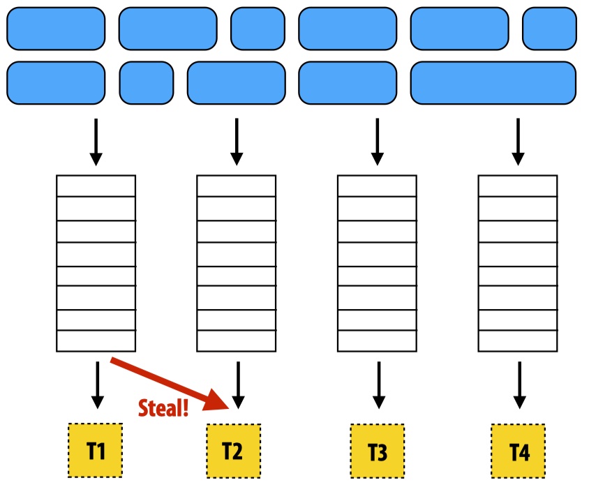
Distributed work queue

Reduce synchronization overhead: if we have m worker threads, and n tasks in a shared work queue, there will be at least n times of synchronization overhead by accessing the single queue. Instead, we can assign the n tasks to m groups first and then put each group to a local queue of every worker. Then workers only need to access their own queues (thus, no synchronization).

When synchronization happens in distributed queues: when a local queue is empty, the worker can communicate and steal tasks from other workers’ queues. This is the only synchronization in a distributed work queue.

Increased locality: workers will also push new tasks to own queues and work on tasks they create (producer-consumer locality).